For the past three months I’ve been working on a Clustered Renderer in OpenGL with the aim of building a framework to experiment with deferred and forward shading techniques. Feel free to check it out on GitHub. I think it’s pretty neat, but I also might be a bit biased. Originally my plan for this post was to write a brief account detailing how I implemented clustered rendering in my engine. However, as the writing went on I increasingly found myself wanting to refer to other efficient algorithms as a way to contextualize the benefits of Clustered Shading. Those references quickly grew into a significant portion of the text, so I decided to split it into two parts.

Part one is a high-level overview of efficient rendering techniques. It follows a simple three-act structure that will take us from classical forward shading all the way to a modern implementation of Clustered Shading. First, I’ll discuss how a given algorithm renders an image. Next, I’ll showcase its major shortcomings and limitations. And lastly, I’ll introduce strategies to overcome those shortcomings, which will segue nicely to the next algorithm. Part two is a deep dive into my own flavor of Clustered Shading, covering all major steps of the algorithm and laying out the specifics of the code I wrote. It’ll also contain some links to further readings on the topic written by developers who have succesfully implemented this technique in high profile games. Let’s get to it!

TL;DR

Clustered shading is an efficient and versatile rendering algorithm capable of using both forward and deferred shading systems. It divides the view frustum into a 3D grid of blocks or “clusters” and quickly computes a list of lights intersecting each active volume.

You can fit this in a tweet!

Part 1:

Efficient Rendering Algorithms

…versatile rendering algorithm capable… …an efficient and… …a list of lights intersecting… …both forward and deferred shading systems… …the view frustum into a 3D grid …

The field of Real-Time rendering has two major opposing driving forces. On the one hand, there’s the strive for realism and a wish for ever improving image quality. On the other hand, there is a hard constraint to deliver those images quickly, usually in less than a 1/30th of a second. The only way to bridge this gap is through the use of software optimizations that allow you to squeeze as much performance as possible from the underlying hardware.

Without these optimizations, it would be impossible to achieve the levels of visual fidelity we are accustomed to in modern high-profile games. So, in a sense, efficient rendering algorithms are at the core of all modern Real-Time rendering processes and are needed to display nearly anything these days. However, of the countless possible optimizations that one could implement, there are a few notable techniques that can have a dramatic impact on performance and have been fully embraced by the graphics community.

We’ll be focusing on two kinds of techniques: those that reduce the amount of unnecessary pixel shader calls and others that focus on lowering the number of lighting computations during shading. You should assume that for most of the algorithms we’ll be discussing all other bottlenecks have already been taken care of. Also, proper culling and mesh management have been performed somewhere further upstream. Other important details that come into play when rendering a mesh will have also been stripped away in favor of presenting a clearer picture of how and why these efficient algorithms outperform their predecessors.

However, there ain’t no such thing as a free lunch. None of these algorithms have zero overhead or are guaranteed to improve the performance of your rendering pipeline. Make sure to consult your ~~primary care phycisian~~ profiler tools to assess the location of your current bottleneck.

Let’s begin by examining the most basic rendering algorithm:

Forward Shading

All animations were built using Blender 2.8, you can find the .blend files here.

//Shaders:
Shader simpleShader

//Buffers:
Buffer display

for mesh in scene
    for light in scene
        display += simpleShader(mesh, light)

In it’s vanilla form, forward shading is a method of rendering scenes by linearly marching forward along the GPU pipeline. A single shader program will be completely in charge of drawing a mesh, starting from the vertex shader, passing through to the rasterizer and finally getting to the fragment shader. The animation and pseudocode above illustrate this behaviour at a glance. For each mesh and light combination we issue a single draw call additively blending the results until the image has been fully assembled. This process is better known as multi-pass forward rendering.

This simple approach leaves a lot of room for improvement, but I wager that it would probably fair fine for simple scenes with a few meshes, basic materials and just a couple of lights. The main issues with this algorithm will become apparent when you increase the quantity or complexity of any of these variables.

For example, a scene with many dynamic lights of different kinds will overwhelm any multi-pass forward renderer due to the combinatorial growth in the number of shader programs. Even though each individual shader is simple, the overhead from shader program switching and bandwidth costs of repeatedly loading meshes becomes a bottleneck quickly. In addition, as you increase the number of meshes you will run into an issue called overdraw. You can see it in action in the animation below.

We begin with the completed scene from the previous animation and then draw new meshes that overlap the previous ones. This invalidates all of the work done shading the covered parts of the background objects. In multi-pass forward rendering this is especially costly, since each completed pixel went through the full vertex-fragment shader pipeline multiple times before being discarded. Alternatively, we could sort the meshes front to back before rendering so that the fragment depth check takes care of the problem. However, sorting meshes based on their screen location is not a trivial problem to solve for large scenes and is costly to do every frame.

What we need instead is a solution that decouples the process of determining if a mesh contributes to the final image from the act of shading a given mesh.

Deferred Shading

Deferred shading is that solution. The idea is that we perform all visibility and material fetching in one shader program, store the result in a buffer, and then we defer lighting and shading to another shader that takes as an input that buffer. As Angelo Pesce discusses in The real-time rendering continuum: a taxonomy there is a lot of freedom as to where we can choose to perform this split. However, the size and content of the intermediate buffer will be determined by the splitting point.

If we’re only concerned with overdraw, the buffer simply has to keep track of the last visible mesh per pixel, normally by recording either its depth or position. Before shading we check if each pixel in a mesh matches the corresponding value recorded in the buffer, if not we discard it. The buffer will be initialized to the far plane depth, that way any mesh that is visible, and therefore closer, will be recorded. To summarize using pseudocode:

//Buffers:
Buffer display
Buffer depthBuffer

//Shaders:
Shader simpleShader
Shader writeDepth

//Visibility
for mesh in scene
    if mesh.depth < depthBuffer.depth
       depthBuffer = writeDepth(mesh)

//Shading and lighting
for mesh in scene
    if mesh.depth == depthBuffer.depth
        for light in scene
            display += simpleShader(mesh, light)

This is commonly known as a Z Pre-pass, and it is considered a mild decoupling of shading and visibility for the sake of reducing the impact of overdraw. And I say reducing instead of eliminating, because overdraw still occurs when you are populating the depth buffer. However, at this point its impact on performance is minimal. This will only hold true if generating geometry and meshes are somewhat straightforward processes in your engine. If meshes come from procedural generation, heavy tessellation or some other source, loading them a second time might negate any possible benefits.

Usually, mentions of Deferred shading refer to a specific system that uses a larger buffer. Within this buffer a series of textures are stored that include information about not only depth, but other shading attributes too. How a deferred system is implemented varies from renderer to renderer, albeit it usually includes material data such as: surface normal, albedo/color or a specular/shininess component. The collection of these textures is commonly referred to as the G-Buffer. If you want to see a specific implementation this Graphics Study by Adrian Courreges goes into detail about how a frame is rendered in Metal Gear Solid V, a fantastic game with a fully deferred rendering engine.

Let’s update our pseudocode and check out how a basic deferred renderer is implemented:

//Buffers:
Buffer display
Buffer GBuffer

//Shaders:
Shader simpleShader
Shader writeShadingAttributes

//Visibility & materials
for mesh in scene
    if mesh.depth < GBuffer.depth
       GBuffer = writeShadingAttributes(mesh)

//Shading & lighting - Multi-pass
for light in scene
    display += simpleShader(GBuffer, light)

Our G-Buffer contains the following shading attributes presented above in a left to right, top to bottom order: surface roughness, normals, albedo and world space position. Notice the differences in material properties between the ico-sphere, the regular sphere and the cube. Lighting is now evaluated for the whole G-Buffer at once instead of per mesh, but still done in a multi-pass fashion.

Deferred shading can also be understood as a tool that allows us to trade off memory bandwidth in exchange for a reduction in computation. In the case of multi-pass setups, the G-Buffer reduces the costs of shading because it can cache vertex transformation results and interpolated shaded attributes, which we later reuse each lighting pass by reading the G-Buffer.

Yet, reading and writing memory is not problem free either. Due to latency, all memory requests take time to be serviced. Even though GPUs can hide this latency by working on some other tasks while waiting, if the ratio of compute operations to memory reads in a program is very low it will eventually have no other option but to stall and wait until the memory delivers on the request. No amount of latency hiding can deal with a program that is requesting data at too high a rate. If you’re interested in understanding why, Prof. Fatahalian’s course on Paralallel Computer architectures covers the modern Multi-core processor architecture, both for CPUs and GPUs, and explains memory latency and throughput oriented systems in detail.

Small Detour: How slow are texture reads anyway?

Texture reads are essentially memory reads and reading memory is always slow. How slow you ask? Well, there is no exact answer since it varies from architecture to architecture, but it is generally considered to be about ~200x slower than a register operation, which we can assume to be on the order of about 0.5ns. A nanosecond is a billionth of a second, hardly a span of time we experience in our day to day lives. Let’s scale it up a bit and imagine that register ops took about a minute instead. In this hellish reality, a memory read would take 3 hours and 20 minutes. Enough time to watch the whole movie The Lord of The Rings: Fellowship of the Ring (extended edition of course) while you wait!

So, why go deferred at all if we’ll be wasting so much time writing data to memory and then reading it again in a second shader program? We’ve already touched upon some of the benefits for multi-pass setups, but in a single-pass setup — shown in the pseudocode below — performance gains happen for different, but much more important, reasons.

//Buffers:
Buffer display
Buffer GBuffer

//Shaders:
Shader manyLightShader
Shader writeShadingAttributes

//Visibility & materials
for mesh in scene
    if mesh.depth < GBuffer.depth
       GBuffer = writeShadingAttributes(mesh)

//Shading & lighting - Single-pass
display = manyLightShader(GBuffer, scene.lights)

In a single-pass setup we evaluate all of the lights in a scene using only a single large shader. This allows us to read the G-Buffer only once and handle all of the different types of lights using dynamic branching. This approach improves upon some of the shortcomings of multi-pass systems by bypassing the need to load shading attributes multiple times. Single-pass shading is also compatible with forward rendering, but can lead to its single shader program — sometimes referred to as “uber-shader” — becoming slow and unwieldy due to its many responsibilities.

And therein lies the biggest perk of deferred shading, it reduces the number of responsibilities of a shader through specialization. By dividing the work between multiple shader programs we can avoid massively branching “uber-shaders” and reduce register pressure — in other words, reduce the amount of variables a shader program needs to keep track of at a given time.

But there are some other drawbacks to classical deferred methods that we haven’t discussed yet. For starters, transparency is problematic because G-Buffers only store the information relevant to a single mesh per pixel. This can be overcome by performing a secondary forward pass for transparent meshes but requires extra work per frame. Another major flaw is that there is no easy way to make use of hardware based anti-aliasing(AA) techniques like Multi-Sampled Anti-Aliasing (MSAA). This is not as big of a deal as it used to be thanks to the progress made in the field of Temporal AA. Lastly, the shading attributes that are stored within the G-Buffer are decided by the shading model that will be used later on in the lighting pass. Varying shading models is costly since it requires either large G-Buffers that can accommodate the data for all models or the implementation of a more complex ID/masking setup.

However, bandwidth bottleneck concerns and large GPU memory usage continues to overshadow all the issues above and remain the major drawbacks to classical deferred systems. An avenue of optimization that we have yet to cover is efficient light culling. So far, for both forward and deferred systems, in both their multi-pass and single-pass variants, we have evaluated lighting for every light at every pixel on the display. This includes pixels that were never in reach of any lights and therefore needlessly issued G-Buffer reads that consumed some of our precious bandwidth. In the next two sections we’ll be looking at ways of efficiently identifying the lights affecting a given pixel.

Tiled Shading & Forward+

With the introduction of Shader Model 5 and DirectX 11 came the compute shader. It opened up the GPU for use as a general-purpose computing tool that provided thread and memory sharing capabilities for programming parallel functions. Compute shaders can be a daunting topic if you’re encountering them for the first time. However, I haven’t been covering implementation details in Part 1 (but I will be in part 2!) so familiarity with compute shaders is not going to be super important moving forward. But, if you are itching to learn about them, I’ve got you covered! Here’s a list of learning sources to get you started.

Compute shaders are heavily used in Tile-based shading to efficiently cull lights for both forward and deferred systems. The idea is that we subdivide the screen into a set of tiles and build up a buffer that keeps track of which lights affect the geometry contained within a tile. Then, during the shading process we evaluate only the lights recorded in a given tile. This significantly reduces the number of lights that need to be evaluated. The animation and pseudocode below illustrate the process:

//Buffers:
Buffer display
Buffer GBuffer
Buffer tileArray

//Shaders:
Shader manyLightShader
Shader writeShadingAttributes
CompShader lightInTile

//Visibility & materials
for mesh in scene
    if mesh.depth < GBuffer.depth
       GBuffer = writeShadingAttributes(mesh)

//Light culling
for tile in tileArray
   for light in scene
      if lightInTile(tile, light)
          tile += light

//Shading
display = manyLightShader(GBuffer, tileArray)

Our starting point is the single-pass deferred algorithm from earlier. Previously, we’d shade each pixel by adding together the individual contributions of each light source, no matter how far away it was from the receiver. This is, technically speaking, the physically correct thing to do since light does have a near infinite area of influence. After all, we do receive light from galaxies that are over 32 billion light-years away. However, because of light attenuation the amount of energy contributed to shading will decrease as a function of distance. Given a spherical light of radius $r$ and intensity $L_i$ , the illumination $I$ at distance $d$ is:

$\begin{equation*} I = \frac{L_i}{(d/r + 1)^2} \end{equation*}$

This allows us to enforce an artificial limit to the area of influence of a light. With enough distance all light sources are attenuated so much that their contributions to shading become effectively imperceptible. We represent this by setting a threshold value of $I$ under which we deem there are no light contributions. This gives light sources a concrete volume of influence which is represented with different shapes for each type of light source. For point lights this volume takes the shape of a sphere, for spotlights a cone and for directional lights a full-screen quad.

In the animation above we represent the volume of influence using colored wire-frame meshes. With these meshes we can perform something akin to collision detection between light volumes and tiles. If any portion of the light “mesh” is contained within a tile, we add that light to a per-tile light list. We perform this check for all tiles and every light in the scene. Finally, we shade the whole scene in one shader pass that uses the per-tile light lists as an input.

Notice that the light culling step does not depend on any other part of the rendering pipeline, hence, we can implement tiled shading using either deferred or a single-pass forward renderer. Tiled forward shading is sometimes also referred to as Forward+, with identical implementation details.

Conceptually, this is all you need to know to grasp the core idea behind tiled shading. Yet you might be wondering about some of the implementation details we have glossed over. For example, how do we determine the optimal size for the tiles? The range of possible sizes goes from one tile per pixel to one tile per screen. You could think of our previous solution as a very inefficient single-tiled system. However, the other end of the spectrum would fare no better. Pixel sized tiles would require large buffers to store and would make the light culling step considerably slower. Not only that, but it wouldn’t even help come shading time since GPUs execute multiple threads —which for now you can imagine as simply being synonymous to pixels — in groups that run exactly the same code for all members. If each thread/pixel in a group has different lights they will want to execute a different code.

When this occurs we say the code has low coherency and is highly divergent. Executing highly divergent code is not what the GPU was designed to do and will cause significant performance degradation. The realization that gets us out of this impasse is that lights tend to affect many pixels at once and these pixels tend to be spatially close together. By tiling our screen we’re leveraging this property and grouping samples together so that they execute the same code. As we discussed above, the GPU is very happy when threads/pixels are coherent and execute exactly the same code. As the saying goes happy GPU, happy you. :)

Hence, achieving the optimal tile size requires finding a balance between making your tiles large, so that execution is coherent, and keeping them small, so that less useless computation is done. Even so, tile size usually ends up being set to the largest thread group of pixels your GPU can manage, even if that means performing many useless calculations per tile. The alternative solution involving smaller tiles would cost us more bandwidth and, as we have seen earlier, bandwidth is a precious resource we don’t want to overspend on. For this reason, we accept a trade off between compute performance for the sake of saving some bandwidth.

Yet, there’s a fairly fundamental problem with tiled shading that comes from an assumption we’ve made above. Let’s look at an example that showcases this issue:

In the animation above we’re looking at the same scene from two perspectives, a familiar front view and an overhead shot that presents the full region of space captured by our virtual camera. In this region, also referred to as view frustum, tiles don’t appear as 2D quads anymore, but as thin and elongated 3D slices of the frustum. As we’ll see soon, this invalidates our previous assumption that tiles contain pixels that are always spatially close together. They might appear next to each other on the screen but, in reality, be separated by a depth discontinuity. In a nutshell, a depth discontinuity is a sudden change in distance, measured from the camera, usually found at the boundaries of one object and another.

Whenever we have an in-front of or behind-of relationship between meshes or lights intersecting a tile, the “spatially close assumption” does not hold true anymore. In the animation above this can be seen with the large smooth sphere at the center. It’s only illuminated by the yellow light located in the midground of the image. Yet, most of the tiles that are responsible for shading the sphere contain more than just the yellow light. In fact, some of them contain all of the lights in the scene! Even though this isn’t quite as bad as our previous situation, we know we can still do better.

A common optimization consists of finding the minimum and maximum depth of the visible meshes in each tile and redefining a tile’s frustum to match this range. For the example above this would be an excellent optimization that would eliminate many unnecessary lights from the center tiles. However, to be able to perform this optimization a Z Pre-pass is necessary, since we have to fill the depth buffer before reading it. As we have already discussed, there are many reasons why this might not be feasible in your rendering pipeline.

Also, this solution does very little to solve the main issue of depth discontinuities within tiles, since the minimum and maximum values will still be dictated by the individual depths of the meshes within. The basic problem is even more fundamental. Tile shading is essentially a 2D concept and the entities we’re trying to represent are 3D. What this means in more practical terms is that light assignment is very strongly view dependent, since it is based on screen space light density. Given different view points within the same scene we might have drastically different shading times and for real time applications unpredictable shading is very undesirable. So, in the next section we’ll be discussing how we can solve this issue and improve upon the basic concepts of tiled shading.

Clustered Shading

Finally, we enter the last stage of our whirlwind tour of Efficient Rendering Algorithms by introducing Clustered Shading. The main idea behind clustered shading will seem like a fairly obvious next step given what we have discussed so far about the shortcomings of tiled shading. Instead of performing light culling checks on 2D screen tiles we’ll do it using 3D cells, also known as clusters. These clusters are obtained by subdivision of the view frustum in the depth axis. Updating the previous scene and our pseudocode we can easily illustrate the process, like so:

//Buffers:
Buffer display
Buffer GBuffer
Buffer clusterArray

//Shaders:
Shader manyLightShader
Shader writeShadingAttributes
CompShader lightInCluster

//Visibility & materials
for mesh in scene
    if mesh.depth < GBuffer.depth
       GBuffer = writeShadingAttributes(mesh)

//Light culling
for cluster in clusterArray
   for light in scene
      if lightIncluster(cluster, light)
          cluster += light

//Shading
display = manyLightShader(GBuffer, clusterArray)

Notice how little has changed in the pseudocode when compared to our tiled implementation. This is actually pretty representative of what happened within my pixel shader when I updated my engine from forward+ to clustered shading. It is certainly a lot more difficult to transform a classic forward/deferred shading pipeline to tiled shading than it is to transition from tiled to clustered.

Regarding the animation, check out the yellow light first. In tiled shading it would have affected tiles that would be responsible for shading the faceted sphere. Yet now, it’s only registering in clusters that are used to shade the smooth sphere in the back. Probably, the biggest difference in this scene is the reduction in number of tiles affected by the red light. Previously, it was affecting all the meshes in the scene, even though it’s only small enough to illuminate the closest sphere and the cube. Now, it is fully contained within one depth slice and only shades those two meshes.

And the best part is that all of this Just Works™ without having to resort to a Z Pre-pass at all, which makes clustered shading compatible with both forward and deferred systems. The key insight is that we know the shape and size of the view frustum before rendering — or it can be easily inferred from basic camera properties — so we can pick a depth subdivision scheme and use that to build a cluster grid that is completely independent of the underlying meshes in the scene.

This is great news since it indicates that we have achieved a strong decoupling of meshes and lighting in the shading process. If with classic forward/deferred our algorithmic complexity was $O(\text{mesh}* \text{lights})$ with clustered shading we have finally achieved a much better performing $O(\text{mesh} + \text{lights})$ algorithm. This is because we now evaluate meshes once, using either deferred or a Z pre-pass, and perform efficient light culling using clustered shading, that makes sure only the relevant lights are considered per mesh.

There are a few other benefits of clustered shading I have yet to mention. For example, since we don’t need any mesh information to build the cluster grid or cull lights we can do this in the CPU instead. This frees up resources on the GPU and can still be made really fast if you make use of SIMD instructions for the culling process. Also, transparent objects are fully supported since the same cluster grid of lights is valid for use in transparent passes. And, if you’re using forward shading, MSAA can be used right out of the box!

As with every algorithm, there are still many improvements that could be made to clustered shading and optimizations I haven’t discussed. We’ll be going into a lot more detail about clustered shading in the second part of this post. So, if you’re curious about the specifics and want to take a look at some implementation details make sure to check it out!

Comparing Algorithms

Even though I’ve presented new techniques as direct replacements to preceding ones, that does not necessarily mean that older algorithms are obsolete. As mentioned in the introduction, no efficient rendering algorithm has zero overhead, and as their degree of refinement increases, so does their complexity. Which of the above algorithms will be best for you will depend on many factors such as: your platform, the number and complexity of lights, triangle count, how your meshes are generated and the complexity of your shading model, among others. I’ve included a table below, taken from Real-Time Rendering 4th edition, that summarizes where the strengths and weaknesses of each technique lie.

	Simple Forward	Simple Deferred	Tile/Clust. Deferred	Tile/Clust. Forward
Geometry Passes	1	1	1	1-2
Light Passes	0	1 / light	1	1
Transparent	yes	no	no	yes
MSAA	yes	no	no	yes
Bandwidth	low	high	medium	low
Register pressure	high	low	possibly low	possibly high
Vary shading	easy	hard	medium	easy

To make the most out of this table it’s best if you have a list of features ordered by priority so you can make an informed decision as to which algorithm best suits your needs. An effective tool for this purpose, that I myself have used in the past, is the Analytical Hierarchy Process (AHP). It helps simplify the decision making process by reducing it into a set of pairwise comparisons and can quantify for you the relative importance of each feature, as well as check how consistent you were in your evaluations.

In the table above, register pressure is analogous to shader complexity and can be an indication of how efficiently an algorithm is making use of GPU compute resources. Transparency and MSAA can actually be supported in both tiled and simple deferred systems but generally at a significantly higher cost when compared to forward. Also, deferred systems are definitely capable of varying shading models/materials, but require use of “shader look up tables” or some material ID system to implement. Given the relative ease with which the same features can be included in a forward engine it was important to highlight the difference.

Lastly, I think it would be worth your time if you factor into your decision making process the current GPU performance trends. In the past, the rate of growth of GPU compute capabilities has continually outpaced memory bandwidth growth. Hence, compute bound algorithms — like tiled or clustered shading — should be of much more interest to us in the future than algorithms bottlenecked by bandwidth. I’m aware that the link I’ve included above might be a bit outdated by now, so take the performance charts with a grain of salt. However, based on what I know about memory, I believe the trend probably still holds true today. But, if you do have any more recent numbers, I would love to take a look at them and maybe use them to update this post.

So, now that I’ve presented the landscape of efficient rendering algorithms I hope that part two of this post we’ll be easier to follow along. I’ll be discussing the details of my own implementation of clustered shading using the compute shader code I wrote for my engine. If you still feel like you need even more background on the topic I’ve included more of the links that I used as a reference while writing this post, and if that doesn’t do the trick, feel free to message me on twitter if you have any questions!

Part 2:

How to Implement Clustered Shading

…and versatile rendering … … and quickly computes a … …a 3D grid of blocks or “clusters” and … …each Active Volume…

Clustered Shading was first introduced by Ola Olsson et al. in “Clustered Deferred and Forward Shading” around 2012. Since then, it has been production proven through implementation in multiple successful projects such as the 2016 reboot of Doom and Detroit: Become Human. It has recently gained more attention due to Unity3D’s announcement that it would be supported in their new High Definition Render Pipeline.

Its popularity is not surprising given that this algorithm offers the highest light-culling efficiency among current real-time many-light algorithms. Moreover, clustered shading improves upon other light culling algorithms by virtue of being compute bound instead of bandwidth limited, which we already discussed the benefit of in part one of this post.

At the heart of this algorithm is the cluster data structure which subdivides the view frustum into a set of volume tiles or clusters. This process can also be viewed as a rough voxelization of the view frustum so, given that volumetric data structures are becoming more popular by the day, this is a great opportunity to become more familiar with them.

The basic steps required to implement clustered shading are outlined in the original paper like so:

Build the clustering data structure.
Render scene to GBuffer or Z Pre-pass.
Find visible clusters.
Reduce repeated values in the list of visible clusters.
Perform light culling and assign lights to clusters.
Shade samples using light list.

My goal for this part is to go through the list in order and explain in detail how I implemented each step. However, steps two and six won’t be covered since they are mostly dependent on the shading model you’re using. Also, steps three and four are combined into one and covered in the section on Determining Active Clusters, much like in Van Oosten’s implementation.

A quick word of warning, most of the code we’ll be looking at from now on will be written in GLSL and aimed for use in compute shaders. Although clustered shading can be fully implemented on the CPU, I personally chose to do it on the GPU. Moving forward, I will assume a basic level of familiarity with compute shaders and shader storage buffer objects. If this is your first time encountering them, I recommend you to take a look at this link, it’s a compilation of the sources I used to learn how to write compute shaders. Also, although most of this code uses OpenGL terminology the principles should directly translate to whatever API you’re using. With all warnings out of the way, let’s begin!

Building a Cluster Grid

There are infinitely many possible ways of grouping view samples together. For rendering, we care mostly about whatever methods help us batch together samples to reduce computations. For example, in Tiled Shading, samples are batched together by screen space proximity, which allows for more efficient lighting evaluations. However, grouping view samples using screen space positions doesn’t account very well for depth discontinuities and leads to very annoying edge cases where a single pixel movement can cause performance issues. Obviously, this is pretty undesirable, so researchers came up with alternative ways to group samples together using either view space position or surface normals.

We’ll be focusing on building cluster grids that group samples based on their view space position. We’ll begin by tiling the view frustum exactly the same way you would in tiled shading and then subdividing it along the depth axis multiple times. There’s no catch-all solution as to how you should perform this depth subdivision and in the original paper the authors discuss three possible ways of doing it.

All animations were built using Blender 2.8, you can find the .blend files here.

The animation above showcases these three alternative subdivision schemes. The first one is regular subdivision in NDC space. As you can see, it’s the most unevenly distributed of the bunch. The clusters close to the far plane are extremely large while the clusters adjacent to the near plane are minuscule. This is due to the non-linearity of NDC space which becomes evident when values get transformed to view space. This article by Nathan Reed helps you visualize this behavior with some very neat plots. This doesn’t quite work as a subdivision scheme because we generally would like our clusters to be small so that they contain very few lights and also evenly distributed, which clearly isn’t the case here.

The next logical step might seem trying to uniformly subdivide in view space, which is what the second image represents. This actually creates the opposite problem. The clusters close to the near plane are now huge while the ones close to the far plane are now wide and very thin which is also No Bueno.

Therefore, the authors of the original paper settled on a non-uniform scheme that is exponentially spaced to achieve self-similar subdivisions, as seen on the third and last image above. The idea is to counteract the NDC non-linearity with another exponential non-linearity. I included the equation used in the paper below. Here, $k$ represents the depth slice, $Z_{vs}$ the view space depth, $\text{near}$ is the near plane depth, $\theta$ represents half the field of view and $S_y$ is equal to the number of subdivision in $y$.

$\begin{equation} k = \left\lfloor\dfrac{ \log\left(-Z_{vs} / \text{near}\right)}{\log\left(1 + \frac{2 tan \theta}{S_y}\right)}\right\rfloor \end{equation}$

Yet, I didn’t end up using any of the above subdivisions in my implementation at all. While researching the topic of clustered shading I found Tiago Sousa’s DOOM 2016 Siggraph presentation and inside spotted the following equation:

$\begin{equation} \text{Z} = \text{Near}_z \left(\frac{\text{Far}_z}{\text{Near}_z} \right)^{\text{slice} / \text{numSlices}} \end{equation}$

Here $Z$ represents depth, $\text{Near}_z$ and $\text{Far}_z$ represent the near and far plane respectively. And slice and numSlices are the current subdivision corresponding to the depth value Z and the total number of subdivisions.

I don’t know about you, but I thought it was pretty neat when I first saw it. You can pretty much visualize the subdivision scheme directly from the math and, more importantly, when you manage to solve for the slice you obtain the following:

$$\begin{equation} \text{slice} = \left\lfloor\ \log\left( Z\right)\frac{\text{numSlices}}{\log\left( \text{Far}_z / \text{Near}_z\right)} - \frac{\text{numSlices} \times \log\left( \text{Near}_z \right)}{\log\left( \text{Far}_z / \text{Near}_z\right)} \right\rfloor \end{equation}$$

The major advantage of equation (3) is that the only variable is Z and everything else is a constant. So, we can pre-calculate both fractions and treat them as a single multiplication and addition, which I refer to as scale and bias in my code. We can now calculate the z slice of any depth value using only a log, a multiplication and an addition operation. I plotted equations (2) and (3) on Desmos and you can play with them by following this link. Or you can also just take a look at the plot below. The view frustum is subdivided into 32 slices with a near plane at 0.3 and a far plane at 100 units.

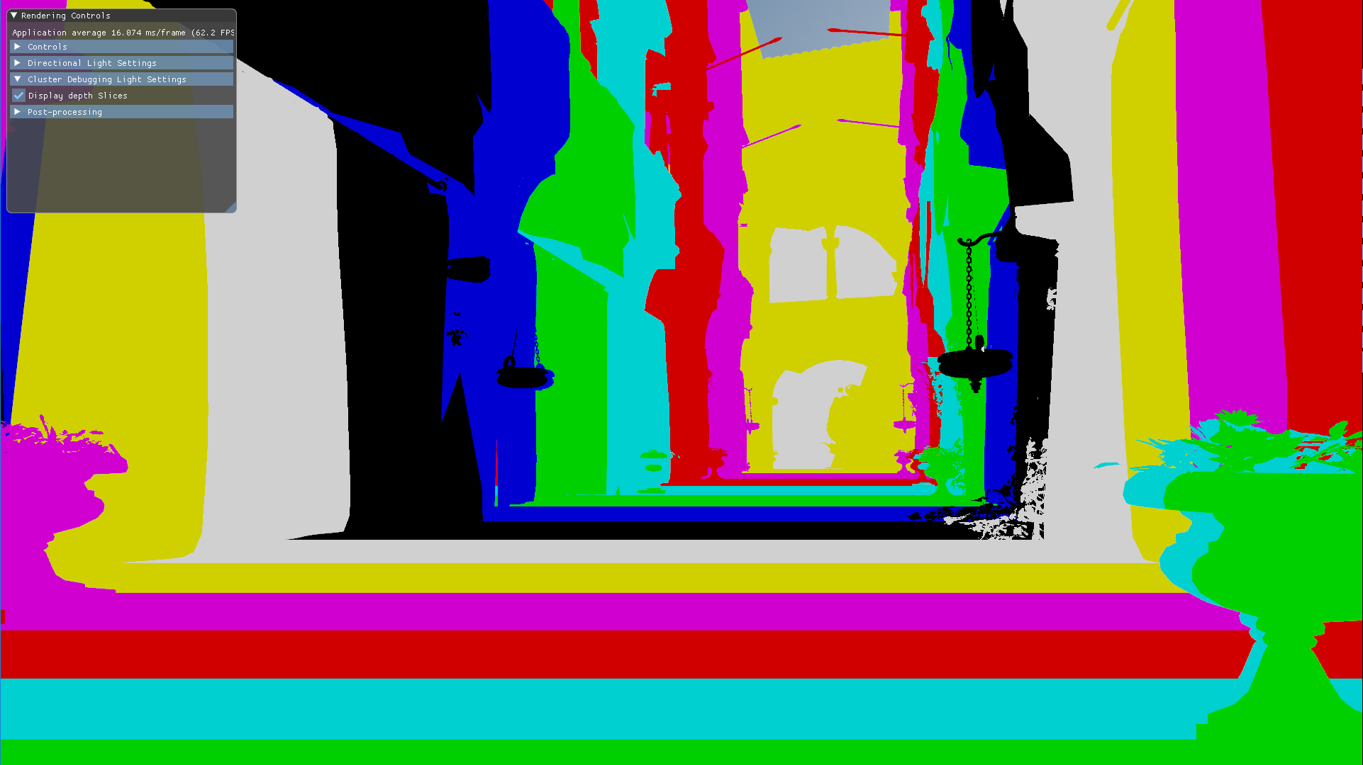
Here’s what the depth slicing looks like in a scene like Sponza, taken directly from my engine. The colors represent the cluster Z index in binary, looping every 8 slices.

Now that we’ve settled for a subdivision scheme, the next thing on our to-do list is figuring out how many subdivisions we’ll use on our cluster grid. The good and bad news is that, once again, this is completely up to you. My advice is that you experiment with different tile sizes and pick a number that isn’t too large. I settled on a 16x9x24 subdivision because it matches my monitors aspect ratio, but it honestly could have been something else. Figuring out what’s an optimal tile size is probably something I should do at some point, and likely a good topic for a future blog post.

One last thing before we move on to the code. We need to decide how we’ll represent the volume occupied by each cluster. We know that we want it to be a simple shape so that the light culling step can be done quickly. And we also would like if it was represented in a compact way so it doesn’t eat up too much bandwidth. An easy solution is to use Axis Aligned Bounding Boxes (AABB) that enclose each cluster. AABBs built from the max and min points of the clusters will be ever so slightly larger than the actual clusters. We’re okay with this since it ensures that there are no gaps in between volumes due to precision issues. Also, AABB’s can be stored using only only two vec3’s, a max and min point.

So, with everything finally in order we can now dig in into the compute shader in charge of building a cluster grid. I had to remove some code to make this fit inside a reasonable amount of space but if you’re interested in seeing the real deal, here’s a link to my code. Let’s take a look:

//Input
uint tileSizePx;  // How many pixels in x does a square tile use
uint tileIndex;   // Linear ID of the thread/cluster
float zFar;       // Far plane distance in view space depth
float zNear;      // Near plane distance in view space depth

//Output
struct cluster{   // A cluster volume is represented using an AABB
   vec4 minPoint; // We use vec4s instead of a vec3 for memory alignment purposes
   vec4 maxPoint;
}
cluster[];        // A linear list of AABB's with size = numclusters

//Each cluster has it's own thread ID in x, y and z
//We dispatch 16x9x24 threads, one thread per cluster
void main(){
    //Eye position is zero in view space
    const vec3 eyePos = vec3(0.0);

    //Per cluster variables
    uint tileSizePx = tileSizes[3];
    uint tileIndex  = gl_GlobalInvocationID;

    //Calculating the min and max point in screen space
    vec4 maxPoint_sS = vec4(vec2(gl_WorkGroupID.x + 1,
                                 gl_WorkGroupID.y + 1) * tileSizePx,
                                 -1.0, 1.0); // Top Right
    vec4 minPoint_sS = vec4(gl_WorkGroupID.xy * tileSizePx,
                            -1.0, 1.0); // Bottom left

    //Pass min and max to view space
    vec3 maxPoint_vS = screen2View(maxPoint_sS).xyz;
    vec3 minPoint_vS = screen2View(minPoint_sS).xyz;

    //Near and far values of the cluster in view space
    //We use equation (2) directly to obtain the tile values
    float tileNear  = -zNear * pow(zFar/ zNear, gl_WorkGroupID.z/float(gl_NumWorkGroups.z));
    float tileFar   = -zNear * pow(zFar/ zNear, (gl_WorkGroupID.z + 1) /float(gl_NumWorkGroups.z));

    //Finding the 4 intersection points made from each point to the cluster near/far plane
    vec3 minPointNear = lineIntersectionToZPlane(eyePos, minPoint_vS, tileNear );
    vec3 minPointFar  = lineIntersectionToZPlane(eyePos, minPoint_vS, tileFar );
    vec3 maxPointNear = lineIntersectionToZPlane(eyePos, maxPoint_vS, tileNear );
    vec3 maxPointFar  = lineIntersectionToZPlane(eyePos, maxPoint_vS, tileFar );

    vec3 minPointAABB = min(min(minPointNear, minPointFar),min(maxPointNear, maxPointFar));
    vec3 maxPointAABB = max(max(minPointNear, minPointFar),max(maxPointNear, maxPointFar));

    //Saving the AABB at the tile linear index
    //Cluster is just a SSBO made of a struct of 2 vec4's
    cluster[tileIndex].minPoint  = vec4(minPointAABB , 0.0);
    cluster[tileIndex].maxPoint  = vec4(maxPointAABB , 0.0);
}

This compute shader is ran once per cluster and aims to obtain the min and max points of the AABB encompassing said cluster. First, imagine we’re looking at the view frustum from a front camera perspective, like we did in the Tiled Shading animations of part one. Each tile will have a min and max point, which in our coordinate system will be the upper right and bottom left vertices of a tile respectively. After obtaining these two points in screen space we set their Z position equal to the near plane, which in NDC and in my specific setup is equal to -1 — I know, I know. I should be using reverse Z, not the default OpenGL layout, I’ll fix that eventually.

Then, we transform these min and max points to view space. Next, we obtain the Z value of the “near” and “far” plane of our target mini-frustum / cluster. And, armed with the knowledge that all rays meet at the origin in view space, a pair of min and max values in screen space and both bounding planes of the cluster, we can obtain the four points intersecting those planes that will represent the four corners of the AABB encompassing said cluster. Lastly, we find the min and max of those points and save their values to the cluster array. And voilà, the grid is complete!

Still, I think it would be worth it to take a look at some of the specific functions that are called inside the compute shader:

//Input:
vec2 screenDimensions;  // Size of the screen in pixels for width and height
mat4 inverseProjection; // The inverse of the projection matrix to get us to view space

//Output:
vec4 view; //The input vector transformed to view space

//Changes a points coordinate system from screen space to view space
vec4 screen2View(vec4 screen){
    //Convert to NDC
    vec2 texCoord = screen.xy / screenDimensions.xy;

    //Convert to clipSpace
    vec4 clip = vec4(vec2(texCoord.x, 1.0 - texCoord.y)* 2.0 - 1.0, screen.z, screen.w);

    //View space transform
    vec4 view = inverseProjection * clip;

    //Perspective projection
    view = view / view.w;

    return view;
}

//Input:
float zDistance; // Normally the z-depth boundaries of a tile
vec3 A,B;        // Two points that are located along the same line

//Output:
vec3 result; //A new point along the same line at the given plane

//Creates a line segment from the eye to the screen point, then finds its intersection
//With a z oriented plane located at the given distance to the origin
vec3 lineIntersectionToZPlane(vec3 A, vec3 B, float zDistance){
    //all clusters planes are aligned in the same z direction
    vec3 normal = vec3(0.0, 0.0, 1.0);
    //getting the line from the eye to the tile
    vec3 ab =  B - A;
    //Computing the intersection length for the line and the plane
    float t = (zDistance - dot(normal, A)) / dot(normal, ab);
    //Computing the actual xyz position of the point along the line
    vec3 result = A + t * ab;
    return result;
}

Specifically, let’s talk about these two functions: line intersection to plane and screen to view. The latter converts a given point in screen space to view space by taking the reverse transformation steps taken by the graphics pipeline. We begin from screen space, transform to NDC space, then clip space and lastly to view space by using the inverse projection matrix and dividing by w. I found this function in Matt Pettineo’s awesomely title blog: THE DANGER ZONE, so thanks Matt!

We use the line intersection to plane function to obtain the points on the corners of the AABB that encompasses a cluster. This function is based on Christer Ericsons implementation of this test from his book Real-Time Collision Detection. The normal vector of the planes is fixed at 1.0 in the z direction because we are evaluating the points in view space and positive z points towards the camera from this frame of reference.

Our list of cluster AABBs will be valid as long as the view frustum stays the same shape. So, it can be calculated once at load time and only recalculated with any changes in FOV or other view field alterning camera properties. My initial profiling in RenderDoc seems to indicate that the GPU can run this shader really quickly, so I think it wouldn’t be a huge deal either if this was done every frame. With our cluster grid assembled we’ve completed step one of our 6 step plan towards building a clustered shading algorithm and can move on to finding visible clusters.

Determining Active Clusters

Technically speaking, this section is optional since active cluster determination is not a crucial part of light culling. Even though it isn’t terribly optimal, you can simply perform culling checks for all clusters in the cluster grid every frame. Thankfully, determining active clusters doesn’t take much work to implement and can speed up the light culling pass considerably. The only drawback is that it will require a Z Pre-pass.

If this isn’t an issue, or you’re using a deferred system, here’s one way you could implement it. The key idea is that not all clusters will be visible all of the time, and there is no point in performing light culling against clusters you cannot see. So, we can check every pixel in parallel for their cluster ID and mark it as active on a list of clusters. This list will most likely be sparsely populated, so we will compact it into another list using atomic operations. Then, during light culling we will check light “collisions” against the compacted list instead, saving us from having to check every light for every cluster. Here’s that process presented more explicitly in code:

//Input
vec2 pixelID; // The thread x and y id corresponding to the pixel it is representing
vec2 screenDimensions; // The total pixel size of the screen in x and y

//Output
bool clusterActive[];

//We will evaluate the whole screen in one compute shader
//so each thread is equivalent to a pixel
void markActiveClusters(){
    //Getting the depth value
    vec2 screenCord = pixelID.xy / screenDimensions.xy;
    float z = texture(screenCord) //reading the depth buffer

    //Getting the linear cluster index value
    uint clusterID = getClusterIndex(vec3(pixelID.xy, z));
    clusterActive[clusterID] = true;
}

//Input
vec3 pixelCoord;  // Screen space pixel coordinate with depth
uint tileSizeInPx; // How many pixels a rectangular cluster takes in x and y
uint3 numClusters; // The fixed number of clusters in x y and z axes

//Output
uint clusterIndex; // The linear index of the cluster the pixel belongs to

uint getClusterIndex(vec3 pixelCoord){
    // Uses equation (3) from Building a Cluster Grid section
    uint clusterZVal  = getDepthSlice(pixelCoord.z);

    uvec3 clusters    = uvec3( uvec2( pixelCoord.xy / tileSizeInPx), clusterZVal);
    uint clusterIndex = clusters.x +
                        numClusters.x * clusters.y +
                        (numClusters.x * numClusters.y) * clusters.z;
    return clusterIndex;
}

These two functions form the first compute shader pass and are equivalent to step three “Find visible clusters.” In function one, markActiveClusters, each thread represents a pixel and its job is to check which cluster it belongs to. Any cluster that we can see is considered active and hence we’ll set it as active in the clusterActive array. The second function, getClusterIndex, is the workhorse of the compute shader. It is responsible for finding which cluster a pixel belongs to using depth and screen space coordinates. To increase efficiency, both Van Oosten and Olsson compact this list into a set of unique clusters.

//Input
bool clusterActive[]; //non-compacted list
uint globalActiveClusterCount; //Number of active clusters

//Output
uint uniqueActiveClusters[]; //compacted list of active clusters

//One compute shader for all clusters, one cluster per thread
void buildCompactClusterList(){
    uint clusterIndex  = gl_GlobalInvocationID;
    if(clusterActive[clusterIndex]){
       uint offset = atomicAdd(globalActiveClusterCount, 1);
       uniqueActiveClusters[offset] = clusterIndex;
    }
}

The globalActiveClusterCount variable keeps track of how many active clusters are currently in the scene and the uniqueActiveClusters array records the indices of those clusters. The buildCompactClusterList compute shader can be run as a separate shader invocation with threads representing clusters and dispatch size equal to the total number of clusters in the scene. Once done, it will output a list of active clusters for us to cull against. We can even launch the next light culling compute shaders indirectly by using the globalActiveClusterCount value as the dispatch size. With this completed, we now have succesfully implemented steps three and four of our original list and we can move on to light culling.

Light Culling Methods

So, with a cluster grid and a list of active clusters ready to go we can finally move on to the most fun part of clustered shading, the light culling step. As a reminder, this step aims to assign lights to each cluster based on their view space position. The main idea is that we perform something very similar to a “light volume collision detection” against the active clusters in the scene and append any lights within a cluster to a local list of lights. I’ve recycled the following animation from part one of this post since I think it does a good job of showcasing the basics of the process:

Performing this “light volume collision detection” requires that I define clearly what I mean by light volume.” In a nutshell, lights become dimmer with distance. After a certain point they are so dim we can assume they aren’t contributing to shading anymore so, we mark those points as our boundary. The volume contained within the boundary is our light volume and if that volume intersects with the AABB of a cluster, we assume that light is contained within the cluster. We’ll be using a pretty common function for testing this I obtained from Crister Ericsons book Real-Time Collision Detection.

//Input:
uint light; // A given light index in the shared lights array
uint tile;  // The cluster index we are testing

//Checking for intersection given a cluster AABB and a light volume
bool testSphereAABB(uint light, uint tile){
    float radius = sharedLights[light].range;
    vec3 center  = vec3(viewMatrix * sharedLights[light].position);
    float squaredDistance = sqDistPointAABB(center, tile);

    return squaredDistance <= (radius * radius);
}

The main idea is that we check the distance between the point light sphere center and the AABB. If the distance is less than the radius they are intersecting. For spotlights, the light volume and consequently the collision tests will be very different. However, I haven’t implemented them in my engine at all so I can’t tell you much about them yet. :( Check out this presentation by Emil Persson that explains how they implemented spotlight culling in Just Cause 3 if you do want to know more.

Our last stop before we begin our step by step breakdown is a quick overview of the data structures we’ll be using. They’re implemented solely on the GPU using shader storage buffer objects, so keep in mind that reads and writes have incoherent memory access and will require the appropriate barriers to avoid any disasters. As we describe them, keep referring back to the following diagram. It will come in handy while you work towards building your own mental picture of how all the pieces fit in together:

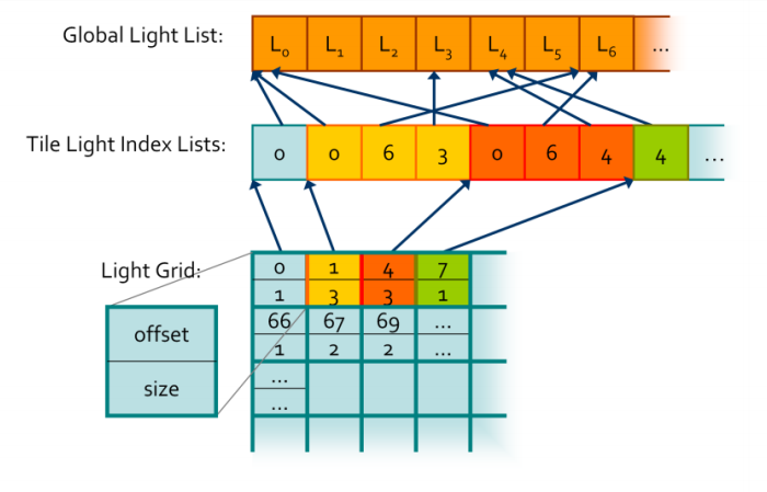
This diagram was made by Ola Olsson and used in his 2014 Siggraph Asia course

We begin by examining the global light list. It is a pretty simple array containing all of the lights in a given scene with a size equivalent to the maximum amount of lights possible in the scene. Every light will have its own unique index based on its location in this array and that index is what we’ll be storing in our second data structure, the global light index list. This array will contain the indices of all of the active lights in the scene grouped by cluster. This grouping is not actually explicit since this array does not contain any information as to how these indices relate to their parent clusters. We store that information in our last data structure, the light grid. This array has as many elements as there are clusters and each element contains two unsigned ints, one that stores the offset to the global light index list and another that contains the number of lights intersecting the cluster.

However, unlike what’s shown in the diagram, the global light index list does not necessarily store the indices for each cluster sequentially. In fact, it might store them in a completely random order. This was a huge source of confusion for me that took way longer than it should have to clear up, so I thought it would be worth mentioning just in case. If you’re wondering why we need such a convoluted data structure, the quick answer is that it plays nicely with the GPU and works well in parallel. Also, it allows both compute shaders and pixel shaders to read the same data structure and execute the same code. Lastly, it is pretty memory efficient since clusters tend to share the same lights and by storing indices to the global light list instead of the lights themselves we save up memory.

Now that we have all the pieces laid out on the board we can take a look at what it takes to cull lights in clustered shading. Because my compute shader would not fit properly in this post I shortened it a bit, if you want to check out the real deal, as always, here’s the link.

//Input
uint threadCount; // Number of threads in a group
uint lightCount;  // Number of total lights in the scene
uint numBatches;  // Number of groups of lights that will be completed
sharedLights[];   // A grouped-shared array which contains all the lights being evaluated

//Output
lightGrid[]; // Array containing offset and number of lights in a cluster
uint globalIndexCount;  // How many lights are active in the scene
globalLightIndexList[]; // List of active lights in the scene

// Runs in batches of multiple Z slices at once
// In my implementation 6 batches
// We begin by each thread representing a cluster
// Then in the light traversal loop they change to representing lights
// Then change again near the end to represent clusters
// NOTE: Tiles actually mean clusters, it's just a legacy name from tiled shading
void main(){
    //Reset every frame
    globalIndexCount = 0;
    uint threadCount = gl_WorkGroupSize.x * gl_WorkGroupSize.y * gl_WorkGroupSize.z;
    uint lightCount  = pointLight.length();
    uint numBatches = (lightCount + threadCount -1) / threadCount;
    uint tileIndex = gl_GlobalInvocationID;

    //Local thread variables
    uint visibleLightCount = 0;
    uint visibleLightIndices[100];

    // Traversing list of lights in batches of equal size to thread
    // group which is equal to 4 slices of the cluster grid at once
    for( uint batch = 0; batch < numBatches; ++batch){
        uint lightIndex = batch * threadCount + gl_LocalInvocationIndex;

        //Prevent overflow by clamping to last light which is always null
        lightIndex = min(lightIndex, lightCount);

        //Populating shared light array
        sharedLights[gl_LocalInvocationIndex] = pointLight[lightIndex];
        barrier();

        //Iterating within the current batch of lights
        for( uint light = 0; light < threadCount; ++light){
            if( sharedLights[light].enabled  == 1){
                //Where the magic happens
                if( testSphereAABB(light, tileIndex) ){
                    visibleLightIndices[visibleLightCount] = batch * threadCount + light;
                    visibleLightCount += 1;
                }
            }
        }
    }

    //We want all thread groups to have completed the light tests before continuing
    barrier();

    //Adding the light indeces to the cluster light index list
    uint offset = atomicAdd(globalIndexCount, visibleLightCount);
    for(uint i = 0; i < visibleLightCount; ++i){
        globalLightIndexList[offset + i] = visibleLightIndices[i];
    }

    //Updating the light grid for each cluster
    lightGrid[tileIndex].offset = offset;
    lightGrid[tileIndex].count = visibleLightCount;
}

In the current version of my cluster shading pipeline I’m not performing any active cluster determination. I wasn’t running a Z Pre-pass until very recently so instead, I’ve chosen to check lights against every cluster of the view frustum. This is also the case in the compute shader above, which performs light culling for every cluster in the cluster grid. The shader is dispatched six times because each thread group contains four z slices $(24/4 = 6)$, which is the largest amount I could comfortably fit inside a single thread group.

Thread groups sizes are actually relevant in this compute shader since I’m using shared GPU memory to reduce the number of reads and writes by only loading each light once per thread group, instead of once per cluster. With that in mind, let’s break down what’s going on within the shader. First, each thread gets its bearings and begins by calculating some initialization values. For example, how many threads there are in a thread group, what it’s linear cluster index is and in how many passes it shall traverse the global light list. Next, each thread initializes a count variable of how many lights intersect its cluster and a local index light array to zero.

Once setup is complete, each thread group begins a traversal of a batch of lights. Each individual thread will be responsible for loading a light and writing it to shared memory so other threads can read it. A barrier after this step ensures all threads are done loading before continuing. Then, each thread performs collision detection for its cluster, using the AABB we determined in step one, against every light in the shared memory array, writing all positive intersections to the local thread index array. We repeat these steps until every light in the global light array has been evaluated.

Next, we atomically add the local number of active lights in a cluster to the globalIndexCount and store the global count value before we add to it. This number is our offset to the global light index list and due to the nature of atomic operations we know that it will be unique per cluster, since only one thread has access to it at any given time. Then, we populate the global light index list by transferring the values from the local light index list (named visibleLightIndices in the code) into the global light index list starting at the offset index we just obtained. Finally, we write the offset value and the count of how many lights intersected the cluster to the lightGrid array at the given cluster index.

Once this shader is done running the data structures will contain all of the values necessary for a pixel shader to read the list of lights that are affecting a given fragment, since we can use the getClusterIndex function from the previous section to find which cluster a fragment belongs to. With this, we’ve completed step five and therefore have all the building blocks in place for a working clustered shading implementation! Of course, I’ll be the first to admit that there is still lots of room for improvement. But even this simple culling method will still manage lights in the order of tens of thousands. If you’re hungry for more, the next section will briefly mention what are some possible optimizations and discuss where you can go read more about them.

Optimization Techniques

There are always improvements that could be made to squeeze that last extra bit of performance out of any rendering algorithm. Although my renderer doesn’t need these yet, I have done some preliminary research on the topic.

If you’re interested, your first stop should be Jeremiah Van Oosten’s thesis where he writes at length about optimizing Clustered Renderers and has links to his testing framework where you can compare different efficient rendering algorithms. In the video below he goes into detail as to how spatial optimization structures like Boundary Volume Hierarchies (BVH) and efficient light sorting can significantly increase performance and allow for scenes with millions of dynamic light sources in real-time.

Ola Olsson, the original author of the paper, gave some talks about clustered rendering around 2014-15. You can find slides for two of them here and here. He and other speakers, present their findings about some various techniques that leverage the benefits of clustered shading. For example, one of them focuses on virtual shadow mapping enabling hundreds of real-time shadow casting dynamic lights, while another presents an alternate clustering method best suited for mobile hardware.

DOOM 2016 is another great source of information. It is considered a milestone implementation of clustered forward shading and many of the advances it made are recorded in this Siggraph 2016 talk by Tiago Sousa and Jean Geffroy. Some interesting takeaways from the talk can be found in the post-processing section. Specifically, in the explanation of how they optimized shaders to make use of GCN scalar units and saved some Vector General-Purpose Registers(VGPR). Also, by voxelizing environment probes, decals and lights the benefits of the cluster data structure were brought over to nearly all items that influence lighting.

Over the coming months, as I continue to work on my renderer, I expect to have to implement some of these techniques to maintain my performance target of 60fps. Right now, it seems that implementing the BVH will be my first task — and specially after how important being familiar with BVH’s will become after Turing. I’ll make sure to write about how that goes and link to it here once the time comes!

Successful Implementations

So I would be remiss not to end this post by sharing some great presentations from other more experienced devs where they discuss their own versions of Clustered shading. As you can imagine, no two are alike, both in the nitty-gritty details of their implementations and in the large scale differences found in the genres of the games they make. It speaks volumes for the flexibility of this algorithm and hints towards a future where hybrid forward/deferred engines are the norm for AAA products that demand the highest visual fidelity.

Also, hey, I’ve technically implemented a Clustered Renderer too! If you’ve forgotten about it after reading this whole post I don’t blame you, but here’s a link so that you don’t have to scroll all the way to the top. It’s a simplified implementation with much of the code commented so you — and me in about a year when I inevitably forget about it — can follow along easily. Okay okay, enough self promotion, here are the goods:

A Primer On Efficient Rendering Algorithms & Clustered Shading.

Table of Contents